Resampling with the Validation Set Approach - An Example in R

Resampling is a technique that allows us to repeatedly draw samples from a set of observations and to refit a model on each sample in order to obtain additional information. Resampling can be useful to estimate the variability of the model fit and to estimate the error rate of the model when applied in new previously unseen data. Resampling can also help in selecting a good level of model flexibility and can also be used to compare the performance (and error rates) of different predictive models.

There are many resampling techniques available. Some of the most popular ones include Cross-Validation techniques (K-Fold, Leave-One-Out, etc.), Bootstrap and Validation Set (training and testing set split).

In this example we’ll focus on one simple technique which will give us the basis for other cross-validation techniques in the future. We’re going to be working with the Validation Set Approach Let’s start by loading the necessary packages. We’ll continue to use Prestige as our dataset of choice. It can be found in the car package library(car):

# Load the packages.
library(car) # where our dataset Prestige resides.
library(rgl)
library(knitr)
library(scatterplot3d)

For illustration purposes, let’s re-create the same data structure we had before with the Prestige dataset:

# Subset the data to capture income, education, women and prestige.
newdata = Prestige[,c(1:4)]

# Center our predictors.
education.c = scale(newdata$education, center=TRUE, scale=FALSE)
prestige.c = scale(newdata$prestige, center=TRUE, scale=FALSE)
women.c = scale(newdata$women, center=TRUE, scale=FALSE)

# Bind these new variables into newdata and display a summary.
new.c.vars = cbind(education.c, prestige.c, women.c)
newdata = cbind(newdata, new.c.vars)
names(newdata)[5:7] = c("education.c", "prestige.c", "women.c" )
summary(newdata)

##    education          income          women           prestige    
##  Min.   : 6.380   Min.   :  611   Min.   : 0.000   Min.   :14.80  
##  1st Qu.: 8.445   1st Qu.: 4106   1st Qu.: 3.592   1st Qu.:35.23  
##  Median :10.540   Median : 5930   Median :13.600   Median :43.60  
##  Mean   :10.738   Mean   : 6798   Mean   :28.979   Mean   :46.83  
##  3rd Qu.:12.648   3rd Qu.: 8187   3rd Qu.:52.203   3rd Qu.:59.27  
##  Max.   :15.970   Max.   :25879   Max.   :97.510   Max.   :87.20  
##   education.c       prestige.c         women.c      
##  Min.   :-4.358   Min.   :-32.033   Min.   :-28.98  
##  1st Qu.:-2.293   1st Qu.:-11.608   1st Qu.:-25.39  
##  Median :-0.198   Median : -3.233   Median :-15.38  
##  Mean   : 0.000   Mean   :  0.000   Mean   :  0.00  
##  3rd Qu.: 1.909   3rd Qu.: 12.442   3rd Qu.: 23.22  
##  Max.   : 5.232   Max.   : 40.367   Max.   : 68.53

The Prestige dataset is a data frame with 102 rows and 6 columns. Each row is an observation that relate to an occupation. The columns relate to predictors such as average years of education, percentage of women in the occupation, prestige of the occupation, etc. Note also that we centered and scaled our data frame and renamed it to newdata.

If you recall from out previous examples, we’ve been focused on creating both simple and multiple linear regression problems with more emphasis on inference without paying too much attention to the predictive quality of the models created. We were simply assessing accuracy and quality of fit on the data used to build these models.

But for any model to have a strong predictive power, we must measure its error rate on data that was not used to build them. When we derive models from a dataset, these models estimate their coefficients by minimizing the errors found exclusively on those data points alone.

If we go on to apply these same models on sets of completely new and previously unseen data points, the model generated may end up yielding large error rates simply because the patterns found in that original dataset may not be picked up in the new dataset.

Error measures that are calculated from the dataset used to build the model (training dataset) are called training dataset error. But, as mentioned, we usually want to use the model results to predict on completely new and previously unseen data points (testing dataset). The error rates estimated from these held-out data points are called testing dataset error.

The Validation Set Approach is a type of method that estimates a model error rate by holding out a subset of the data from the fitting process (creating a testing dataset). The model is then built using the other set of observations (the training dataset). Then the model result is applied on the testing dataset in which we can then calculate the error (testings dataset error). In summary, this general idea allows for the model to not overfit.

Let’s illustrate with an example from our newdata dataframe:

set.seed(7)
# Create a training and a test dataset with 50% of the data in the training set.
trainRows = sample(1:nrow(newdata),0.5*nrow(newdata))
length(trainRows)

## [1] 51

Note from the above code that we created a training and a testing dataset. We’ll be using the training dataset to build our predictive model and then applying it on the testing dataset to assess the error rate. Since our target variable (income from the Prestige dataset) is of a continuous nature, we’ll continue to apply linear regression models for now. Consequently, our error rate will be given by a continuous variable error measure such as the Mean Squared Error or the Root Mean Squared Error.

Before we fit a linear model in our dataset, let’s examine how our predictors are related to our target variable income:

# Plot matrix of all variables.
plot(newdata[,c(1:4)], pch=16, col="blue", main="Matrix Scatterplot of Income, Education, Women and Prestige")

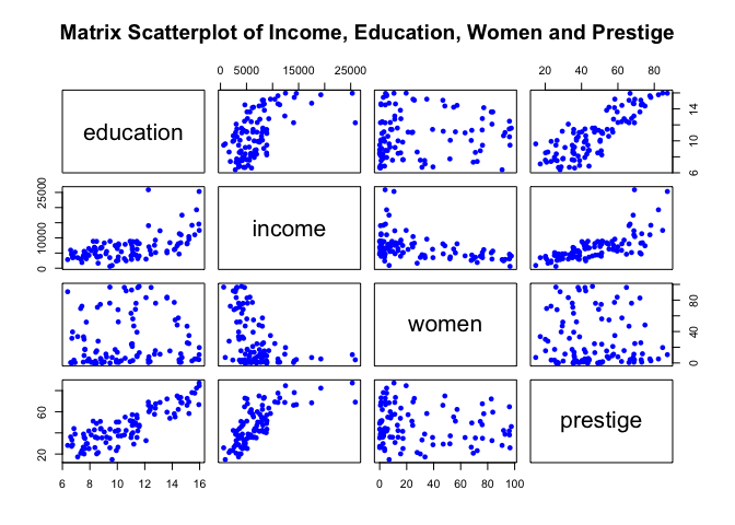
Remember from our previous examples, we decided to manually exclude education from our multiple regression analysis as it was overfitting the data (note from the plot above how similar education’s pattern is relative to prestige’s pattern) and was not adding a significant p-value when prestige was also present in the data. So we went on to generate a few models containing these two predictors only.

For simplicity sake, let’s fit a random multiple linear model with both prestige and women as predictors:

# Fit a model in the training data with income as our response and the predictors as prestige and women.
mod1 = lm(income ~ prestige.c + women.c , data=newdata[c(trainRows), ])
summary(mod1)

## 
## Call:
## lm(formula = income ~ prestige.c + women.c, data = newdata[c(trainRows), 
##     ])
## 
## Residuals:
##     Min      1Q  Median      3Q     Max 
## -3926.3 -1001.3  -281.7   968.6 10519.8 
## 
## Coefficients:
##             Estimate Std. Error t value Pr(>|t|)    
## (Intercept)  6806.90     324.45  20.980  < 2e-16 ***
## prestige.c    175.50      18.41   9.534 1.18e-12 ***
## women.c       -48.70      11.11  -4.382 6.36e-05 ***
## ---
## Signif. codes:  0 '***' 0.001 '**' 0.01 '*' 0.05 '.' 0.1 ' ' 1
## 
## Residual standard error: 2314 on 48 degrees of freedom
## Multiple R-squared:  0.711,  Adjusted R-squared:  0.699 
## F-statistic: 59.06 on 2 and 48 DF,  p-value: 1.148e-13

# Plot residuals.
par(mfrow=c(2,2))
plot(mod1, pch=16)

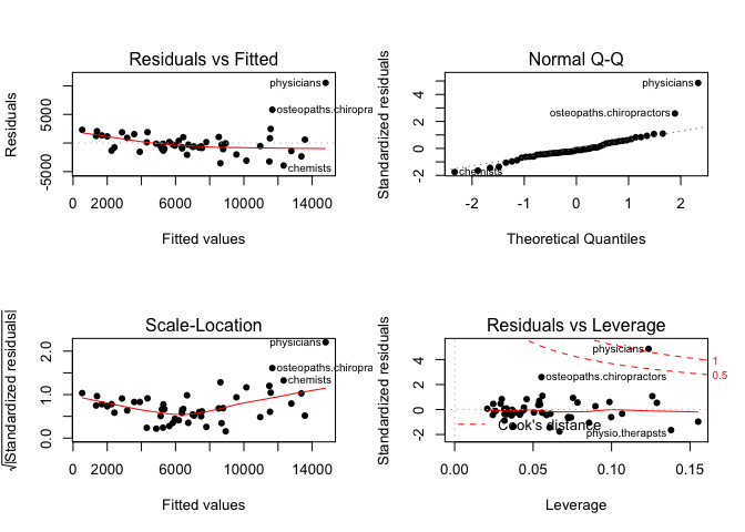
We fit a linear model using lm function. Observe we subset our data for the model to learn only from the training set. The resulting model shows significant p-values for the predictors and the model overall. Both our F-statistic our Adjusted R-squared are not great. Our Residual Standard Error is relatively high. The residual plots also highlight the present of some outliers.

Let’s inspect the model fit on the observed data in an interactive 3D plot (you can click and drag the graph around to change the viewing angle):

newdat <- expand.grid(prestige.c=seq(-35,45,by=5),women.c=seq(-25,70,by=5))
newdat$pp <- predict(mod1,newdata=newdat)
with(newdata,plot3d(prestige.c,women.c,income, col="blue", size=1, type="s", main="3D Linear Model Fit"))
with(newdat,surface3d(unique(prestige.c),unique(women.c),pp,
                      alpha=0.3,front="line", back="line"))

You must enable Javascript to view this page properly.

Note how the model plane fits relatively well around the lower section of the income scale but given a handful of outliers, we end up having a relatively weak linear relationship. Let’s now - to keep in line with the objective of this example - simply apply the model onto the testing dataset (those observations we’ve previously reserved to test how well the model would fit on unused data):

# Predict on the testing dataset and calculate Root Mean Squared Error. 
sqrt(mean((newdata$income-predict(mod1, newdata))[-trainRows]^2))

## [1] 2804.979

Note from the above code that we use the predict function to apply the model onto the testing set. The results calculate the Root Mean Squared Error (RMSE). The Root Mean Squared Error is simply the square root of the average squared errors found between the actual data point and the model fitted values. Taking the square root allows the error to have the same units as the quantity being estimated in the Y axis which yields a more easily interpretable result. The Root Mean Squared Error measure tends to be influenced by variances due to outliers (which is our case here since we got a RMSE of $2,805). RMSE is most useful when large errors are not desired. We could have used another measure such as Mean Absolute Error which measures the average value of the errors between the prediction and the actual data giving similar weight to all error values.

So up to now, we’ve seen that the Validation Set approach provides a simple estimate of the test error rate (applying the model on previously unseen data). However, if we run the training and testing split with a different set of data for each sample, we will obtain somewhat different errors on the testing set. Let’s see how this plays out in the dataset. We’ll create a for loop to generate 100 sample sets for train and test with the model and see how the Root Mean Squared Error varies:

set.seed(5)

rmse=c()

for(i in 1:100){
  train = sample(1:nrow(newdata),0.5*nrow(newdata))
  test = setdiff(1:nrow(newdata),train)
    mods <- lm(income ~ prestige.c + women.c, data=newdata[train, ])
    preds = predict(mods,newx=newdata[test,])
    rmse[i] = sqrt(mean((newdata$income-predict(mods, newdata))[test]^2))
    # cat(rmse[length(rmse)],'\n') # you can uncomment this line if you want to see all values printed out.
}

mean(rmse)

## [1] 2597.934

# Plot histogram of scores.
hist(rmse, density=35, main = "Test RMSE over 100 Samples", xlab = "Value of Obtained RMSE", col="blue", border="black")
abline(v=mean(rmse), lwd=3, col="red")

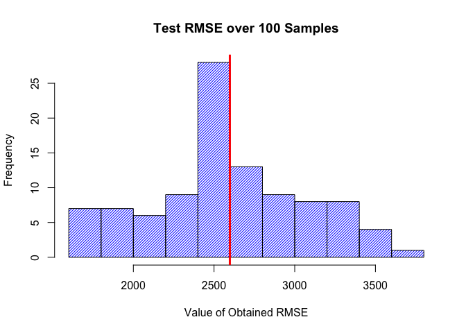
The histogram above highlights (the vertical red line) the average RMSE across 100 different samples as well as the spread in which the RMSE can reach. The RMSE of the income variable we got from this resampling example ranges from $1,606 to $3,695. These are moderately high RMSE values.

These results ultimately show us how the linear model fit is not appropriate in this case. It also shows that despite the fact the validation set approach is simple to implement, it can be highly variable depending on which observations are part of either the training or the testing datasets.

From here we could try to include a quadratic term on the predictors and a transformation for the target variable income - as we did in previous examples - to see how better the model would fit the data. But for brevity sake, we’ll leave it as is for now.

In future examples, we’ll see other techniques such as cross-validation and bootstrap which attempt to address the issues of variability in the training / testing sample due to the existence of fewer observations in which the model is trained on. We’ll also illustrate an example of a classification problem.

You May Also Like...