Intro to Classification Problems: Simple Logistic Regression for Churn Modelling
When we study approaches for predicting qualitative responses, we study classification problems.
19 mins reading time
In many situations in statistical learning, the response variable you want to predict in your dataset is not quantitative (for example, height or weight of individuals). Sometimes, the response variable is instead qualitative (Female / Male are an example of a qualitative data).
When we study approaches for predicting qualitative responses, we study classification problems. Classification because, in these situations, we are in fact classifying an observation, and allocating it to a specific class or category (is it Female or Male?, is it Blue, Red or Green?, etc.).
There are many classification techniques used to predict a qualitative response. Some of the most common ones are Logistic Regression, Linear Discriminant Analysis and K-Nearest neighbors. There are also some relatively more advanced classifiers such as Classification Trees, Random Forests, Boosting, Support Vector Machines and others.
In this example, we’ll briefly touch on one single technique, the Simple (one predictor) Logistic Regression method with a binary dependent variable (when the dependent variable has more than two classes, we refer to multinomial logistic regression). Logistic Regression is a technique that attempts to models the probability of a given qualitative variable, generally in a binary form.
For this Simple Logistic Regression example, we’re going to work with a publicly available telco dataset that is very interesting for this approach. The dataset was sourced from the MLC++ library of the sgi website under the tech archives.
Let’s start by loading the necessary packages and downloading the dataset:
# Load libraries
library(ggplot2)

# load both the variable names file and the variable values file
varNms = read.csv("http://www.sgi.com/tech/mlc/db/churn.names",
               skip=4, header=FALSE,
               sep=":", colClasses=c("character", "NULL"))[[1]]

print(varNms)
##  [1] "state"                         "account length"
##  [3] "area code"                     "phone number"
##  [5] "international plan"            "voice mail plan"
##  [7] "number vmail messages"         "total day minutes"
##  [9] "total day calls"               "total day charge"
## [11] "total eve minutes"             "total eve calls"
## [13] "total eve charge"              "total night minutes"
## [15] "total night calls"             "total night charge"
## [17] "total intl minutes"            "total intl calls"
## [19] "total intl charge"             "number customer service calls"
dt = read.csv("http://www.sgi.com/tech/mlc/db/churn.all",
              header=FALSE, col.names=c(varNms,"churn"))
print(head(dt))
##   state account.length area.code phone.number international.plan
## 1    KS            128       415     382-4657                 no
## 2    OH            107       415     371-7191                 no
## 3    NJ            137       415     358-1921                 no
## 4    OH             84       408     375-9999                yes
## 5    OK             75       415     330-6626                yes
## 6    AL            118       510     391-8027                yes
##   voice.mail.plan number.vmail.messages total.day.minutes total.day.calls
## 1             yes                    25             265.1             110
## 2             yes                    26             161.6             123
## 3              no                     0             243.4             114
## 4              no                     0             299.4              71
## 5              no                     0             166.7             113
## 6              no                     0             223.4              98
##   total.day.charge total.eve.minutes total.eve.calls total.eve.charge
## 1            45.07             197.4              99            16.78
## 2            27.47             195.5             103            16.62
## 3            41.38             121.2             110            10.30
## 4            50.90              61.9              88             5.26
## 5            28.34             148.3             122            12.61
## 6            37.98             220.6             101            18.75
##   total.night.minutes total.night.calls total.night.charge
## 1               244.7                91              11.01
## 2               254.4               103              11.45
## 3               162.6               104               7.32
## 4               196.9                89               8.86
## 5               186.9               121               8.41
## 6               203.9               118               9.18
##   total.intl.minutes total.intl.calls total.intl.charge
## 1               10.0                3              2.70
## 2               13.7                3              3.70
## 3               12.2                5              3.29
## 4                6.6                7              1.78
## 5               10.1                3              2.73
## 6                6.3                6              1.70
##   number.customer.service.calls   churn
## 1                             1  False.
## 2                             1  False.
## 3                             0  False.
## 4                             2  False.
## 5                             3  False.
## 6                             0  False.
Note the dataset was provided with the values separated from the variable names. We load them both separately and directly from the host using the read.csv function. From the variable names file we can see that the target variable name does not exist, so we manually create it (churn).
By inspecting the dataset we can see that it seems to be on an individual telco account level and bringing different features such as account length, area code, presence of international plan, voicemail, and other usage dimensions.
Let’s create a train and test set for this data so we can train our model and then test on previously unseen data. For this simple logistic regression example, we’ll keep only the Number of Customer Service Calls as our predictor and churn as our response variable:
# shorten number of features for simplicity
dt = dt[c(20, 21)]

# recode target variable into zeros and ones
dt$churn = ifelse(as.numeric(dt$churn) == 1, 0,
                  ifelse(as.numeric(dt$churn) == 2, 1,NA))

# create a train and test set with a sample of 75%
# of the 5000 records as train and 25% as test.
set.seed(123)
trainRows = sample(1:nrow(dt), 0.75*nrow(dt))
tr_dt = dt[trainRows, ]
te_dt = dt[-trainRows, ]

# inspect data frame
str(tr_dt)
## 'data.frame':	3750 obs. of  2 variables:
##  $ number.customer.service.calls: int  4 1 0 1 4 2 3 1 3 1 ...
##  $ churn                        : num  0 0 0 0 0 0 0 0 0 0 ...
summary(tr_dt)
##  number.customer.service.calls     churn
##  Min.   :0.000                 Min.   :0.0000
##  1st Qu.:1.000                 1st Qu.:0.0000
##  Median :1.000                 Median :0.0000
##  Mean   :1.542                 Mean   :0.1416
##  3rd Qu.:2.000                 3rd Qu.:0.0000
##  Max.   :9.000                 Max.   :1.0000
Now we have it. A train dataset with 3,750 telecom customer accounts in which we’ll train our simple logistic regression model across a feature we think could be useful to help explain why customers churned. We’ve also recoded the target variable into 2 levels: 0 (did not churn) and 1 (did churn).
By creating a histogram of our predictor variable Number of Customer Service Calls we can examine its skeweness:
# Histogram of Number of Customer Service Calls
qplot(number.customer.service.calls, data = tr_dt, geom="histogram", binwidth=1) +
  labs(title = "Historgram of Number of Customer Service Calls") +
  labs(x ="Number of Customer Service Calls") +
  labs(y = "Frequency of Number of Accounts") +
  scale_y_continuous(breaks = c(0,100,200,300,400,500,600,700,800,900,1000,1100,1200,1300, 1400, 1500), minor_breaks = NULL) +
  scale_x_continuous(breaks = c(0,1,2,3,4,5,6,7,8,9), minor_breaks = NULL) +
   geom_vline(xintercept = mean(tr_dt$number.customer.service.calls), show.legend=TRUE, color="red") +
  geom_vline(xintercept = median(tr_dt$number.customer.service.calls), show.legend=TRUE, color="blue")
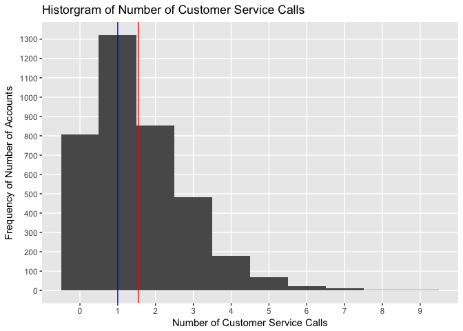
Accounts from this training data set make an average of 1.5424 calls, with the median value sitting at 1 calls. Note also how the shape of the data is relatively right skewed.
For this dataset, logistic regression will model the probability a customer will churn. So considering the predictor Number of Customer Service Calls - which here we are assuming it relates to the number of calls an account made to customer service centre to complain about something - the probability of churn is given by:
Pr(churn = yes given Number of Customer Service Calls)
And this probability will range between 0 and 1 (and nothing outside of these values). So for any range of account length value, a prediction can be made for churn.
The logistic function is given by:
\[p(X)=\frac{e^{B0+B1*X}}{1+e^{B0+B1*X}}\]As with linear models, here our regression coefficients B0 and B1 are unknowns and need to be estimated. Differently than linear regressions though, we use a method called maximum likelihood which tries to find the parameters such that the estimates yield a number close to 1 (one) for all individuals who churned and a number close to 0 (zero) for all individuals who did not churn. The estimated B0 and B1 values are chosen to maximise this likelihood.
To illustrate, let’s jump right into fitting the logistic model and plot the function with the estimated probabilities of churn given our predictor variable Number of Customer Service Calls. We’ll use glm() function which fits generalized linear models, including logistic regression. We’ll plot the logistic function using ggplot2:
# fit a logistic model on the training set using one predictor
set.seed(7621)
mod1 = glm(churn ~ number.customer.service.calls, data=dt, family=binomial, subset=trainRows)

# inspect model
summary(mod1)
##
## Call:
## glm(formula = churn ~ number.customer.service.calls, family = binomial,
##     data = dt, subset = trainRows)
##
## Deviance Residuals:
##     Min       1Q   Median       3Q      Max
## -1.4645  -0.5749  -0.4780  -0.3959   2.2738
##
## Coefficients:
##                               Estimate Std. Error z value Pr(>|z|)
## (Intercept)                   -2.50666    0.08181  -30.64   <2e-16 ***
## number.customer.service.calls  0.39504    0.03305   11.95   <2e-16 ***
## ---
## Signif. codes:  0 '***' 0.001 '**' 0.01 '*' 0.05 '.' 0.1 ' ' 1
##
## (Dispersion parameter for binomial family taken to be 1)
##
##     Null deviance: 3058.9  on 3749  degrees of freedom
## Residual deviance: 2916.8  on 3748  degrees of freedom
## AIC: 2920.8
##
## Number of Fisher Scoring iterations: 4
# plot logistic function with the estimated probabilities using ggplot2
ggplot(tr_dt, aes(x=number.customer.service.calls, y=churn)) +
  geom_point() +
  labs(title = "Model Fit for Churn given the Number of Customer Service Calls") +
  labs(x ="Number of Customer Service Calls") +
  labs(y = "Churn - Probability Estimates - 0=No | 1=Yes") +
  geom_smooth(method = "glm", method.args = list(family = "binomial")) +
  scale_y_continuous(breaks = c(0.0, 0.1,0.2,0.3,0.4,0.5,0.6,0.7,0.8,0.9,1.0), minor_breaks = NULL) +
  scale_x_continuous(breaks = c(0:9), minor_breaks = NULL) +
  geom_hline(yintercept = 0.5, show.legend=TRUE, color="red") +
  annotate("text", x = 2, y = 0.52, label = "Moment Probability to Churn goes beyond 50%", size=3, col="red")
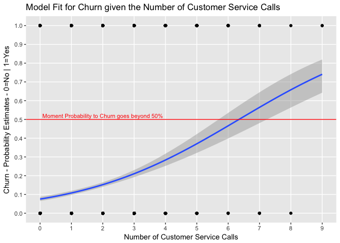
Let’s look at both the model output and the plot above:
-
We initially fit a logistic regression model using the generalized linear model function to predict churn relative to the number of customer service calls using glm() with the binomial family. Generalized linear models are an adaptation of the linear regression model which allows for the response variable to have distributions other than the normal distribution. Each outcome of the response variable, in this case, churn is assumed to be generated from a particular distribution in the exponential family (binomial, gamma, Poisson, etc.)
-
The model output table shows somewhat similar structure to the ones we’ve seen in linear regression. Note the response variable (churn) is in log odds, so the coefficient of Number of Customer Service Calls can be interpreted as “for every additional customer service call made by an account, the odds of that account will churn increases by $e^{B1}$ = 1.4844369 times”.
-
Both the Null deviance and Residual deviance help us assess model performance. Null deviance shows how well the response (churn) is predicted by a model with nothing but an intercept. The number is pretty high and indicates a poor fit. The Residual deviance shows how well the response is predicted by the model when the predictor Number of Customer Service Calls is included. Here we see that the decline in deviance is an evidence of an improved model fit. (One could argue the difference is really not significant.)
-
The p-values associated with our coefficient estimates are pretty small. We can also check for the accuracy of the coefficient estimates by computing their standard errors. For example, the z-statistic values associated with B1 is $\frac{B1}{SE(B1)}$. So in our case, we can be somewhat confident that there is an association between Number of Customer Service Calls and the probability of churn.
-
With the coefficients now estimated, we can compute the probability of churn for any given Number of Customer Service Calls made. So, for example, using the coefficient estimates from the table we can predict that the churn probability for an account that made 6 calls to Customer Service is:
We can also write a customised function in R to help us calculate any given number of calls made one at a time and check the probability a customer will churn given that number of customer service calls made:
# function that generates the probability to churn  given a value of number of calls made
prob_x <- function(x){
  e = 2.71828
	b0 = summary(mod1)$coefficients[1]
	b1 = summary(mod1)$coefficients[2]

	result = (e^(b0+b1*x))/(1+(e^(b0+b1*x)))
	return(result)
}

# ask the function to give you the probability to churn given there were 6 calls made
prob_x(6)
## [1] 0.4659403
So from the code above you can see the function arrives in the same probability values as per the formula. You can try this function with any other number to see it output the probabilities.
-
Now looking at the logistic function plot above we can see that because the relationship between p(X) and X is not a straight line (see the blue fitted line looks more like an S-Shaped or Sigmoid curve), the value of B1 does not correspond to the change in p(X) given a one-unit increase in X. The amount p(X) changes in X will depend on the current value of X. Increasing X by one unit changes the log odds by B1 (or multiplies the odds by $e^{B1}$). Also, the shaded grey area indicates the Standard Error for each value of X.
-
From the plot we can also infer that the fitted blue line does go too close to 1 in the scale. One can think that the reason for that is also that there are a number of customers which have not churned (churn value is zero) but that have made a high number of calls. Inversely, it’s clear that customers whom have actually churned did not make only 1 or 2 Customer Service Calls.
With our model generated, we can now use the predict() function to predict the probability that each account will churn given their Number of Customer Service Calls:
# Generate a prediction on the held out / test data set
set.seed(825)
churn_prob = predict(mod1, te_dt, type="response")


# Compare predictions with actual values
churn_pred = rep(0, 1250)
churn_pred[churn_prob>.5]=1

# create a confusion matrix
table(churn_pred, te_dt$churn)
##
## churn_pred    0    1
##          0 1073  175
##          1    1    1
mean(churn_pred==te_dt$churn)
## [1] 0.8592
After fitting a logistic regression on our training set (mod1) we obtain the predicted probabilities of the accounts to churn form our test set. We finally compare the models predictions with the actual churn results in the test dataset.
A confusion matrix is a helpful tool to assess the errors the model is making. For example, the table above reveals that our simple logistic regression model predicted a total of only 2 accounts would churn (out of our 1,250 test set). Of these 2 accounts, 1 actually churned and another did not. So only 1 out of 1,074 accounts who did not churn, were incorrectly classified. This looks like a pretty low error rate! Looking further though, of the 176 accounts who actually churned, 175 of them (or almost all of them) were not correctly classified by our simple logistic model. So while the overall error rate is quite low, the error rate for accounts who churned is pretty high.
In this example, we touched on a brief introduction to classification problems with a simple logistic regression model. We created a simple prediction approach to illustrate a classifier. Finally, we assess the model accuracy using the confusion matrix (further terms that assess performance of a classifier such as sensitivity and specificity were purposely not discussed.)
In another example, we’ll cover some other classification techniques, look at some further performance metrics to assess model accuracy and start looking at The Bayes’ theorem for more advanced classification models (LDA, QDA, etc.).