Using R for a Simple K-Means Clustering Exercise
K-Means is a clustering approach that belogs to the class of unsupervised statistical learning methods.
11 mins reading time
K-Means is a clustering approach that belogs to the class of unsupervised statistical learning methods. K-Means is very popular in a variety of domains. In biology it is often used to find structure in DNA-related data or subgroups of similar tissue samples to identify cancer cohorts. In marketing, K-Means is often used to create market/customer/product segments.
The general idea of a clustering algorithm is to partition a given dataset into distinct, exclusive clusters so that the data points in each group are quite similar to each other.
One of the first steps in building a K-Means clustering work is to define the number of clusters to work with. Subsequently, the algorithm assigns each individual data point to one of the clusters in a random fashion. The underlying idea of the algorithm is that a good cluster is the one which contains the smallest possible within-cluster variation of all observations in relation to each other. The most common way to define this variation is using the squared Euclidean distance. This process of identifying groups of similar data points can be a relatively complex task since there is a very large number of ways to partion data points into clusters.
Generally, the way K-Means algorithms work is via an iterative refinement process:
1.Each data point is randomly assigned to a cluster (number of clusters is given before hand). 2.Each cluster’s centroid (mean within cluster) is calculated. 3.Each data point is assigned to its nearest centroid (iteratively to minimise the within-cluster variation) until no major differences are found.
Let’s have a look at an example in R using the Chatterjee-Price Attitude Data from the library(datasets) package. The dataset is a survey of clerical employees of a large financial organization. The data are aggregated from questionnaires of approximately 35 employees for each of 30 (randomly selected) departments. The numbers give the percent proportion of favourable responses to seven questions in each department. For more details, see ?attitude.
# Load necessary libraries
library(datasets)

# Inspect data structure
str(attitude)
## 'data.frame':	30 obs. of  7 variables:
##  $ rating    : num  43 63 71 61 81 43 58 71 72 67 ...
##  $ complaints: num  51 64 70 63 78 55 67 75 82 61 ...
##  $ privileges: num  30 51 68 45 56 49 42 50 72 45 ...
##  $ learning  : num  39 54 69 47 66 44 56 55 67 47 ...
##  $ raises    : num  61 63 76 54 71 54 66 70 71 62 ...
##  $ critical  : num  92 73 86 84 83 49 68 66 83 80 ...
##  $ advance   : num  45 47 48 35 47 34 35 41 31 41 ...
# Summarise data
summary(attitude)
##      rating        complaints     privileges       learning
##  Min.   :40.00   Min.   :37.0   Min.   :30.00   Min.   :34.00
##  1st Qu.:58.75   1st Qu.:58.5   1st Qu.:45.00   1st Qu.:47.00
##  Median :65.50   Median :65.0   Median :51.50   Median :56.50
##  Mean   :64.63   Mean   :66.6   Mean   :53.13   Mean   :56.37
##  3rd Qu.:71.75   3rd Qu.:77.0   3rd Qu.:62.50   3rd Qu.:66.75
##  Max.   :85.00   Max.   :90.0   Max.   :83.00   Max.   :75.00
##      raises         critical        advance
##  Min.   :43.00   Min.   :49.00   Min.   :25.00
##  1st Qu.:58.25   1st Qu.:69.25   1st Qu.:35.00
##  Median :63.50   Median :77.50   Median :41.00
##  Mean   :64.63   Mean   :74.77   Mean   :42.93
##  3rd Qu.:71.00   3rd Qu.:80.00   3rd Qu.:47.75
##  Max.   :88.00   Max.   :92.00   Max.   :72.00
As we’ve seen, this data gives the percent of favourable responses for each department. For example, in the summary output above we can see that for the variable privileges among all 30 departments the minimum percent of favourable responses was 30 and the maximum was 83. In other words, one department had only 30% of responses favourable when it came to assessing ‘privileges’ and one department had 83% of favourable responses when it came to assessing ‘privileges’, and a lot of other favourable response levels in between.
When performing clustering, some important concepts must be tackled. One of them is how to deal with data that contains multiple (or more than 2) variables. In such cases, one option would be to perform Principal Component Analysis (PCA) and then plot the first two vectors and maybe additionally apply K-Means. Other checks to be made are whether the data in hand should be standardized, whether the number of clusters obtained are truly representing the underlying pattern found in the data, whether there could be other clustering algorithms or parameters to be taken, etc. It is often recommended to perform clustering algorithms with different approaches and preferably test the clustering results with independent datasets. Particularly, it is very important to be careful with the way the results are reported and used.
For simplicity, we’re not going to tackle most of these concerns in this example but they should always be part of a more robust work.
In light of the example, we’ll take a subset of the attitude dataset and consider only two variables in our K-Means clustering exercise. So imagine that we would like to cluster the attitude dataset with the responses from all 30 departments when it comes to ‘privileges’ and ‘learning’ and we would like to understand whether there are commonalities among certain departments when it comes to these two variables.
# Subset the attitude data
dat = attitude[,c(3,4)]

# Plot subset data
plot(dat, main = "% of favourable responses to
     Learning and Privilege", pch =20, cex =2)
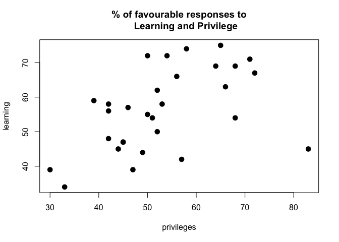
With the data subset and the plot above we can see how each department’s score behave across Privilege and Learning compare to each other. In the most simplistic sense, we can apply K-Means clustering to this data set and try to assign each department to a specific number of clusters that are “similar”. Let’s use the kmeans function from R base stats package:
# Perform K-Means with 2 clusters
set.seed(7)
km1 = kmeans(dat, 2, nstart=100)

# Plot results
plot(dat, col =(km1$cluster +1),
     main="K-Means result with 2 clusters", pch=20, cex=2)
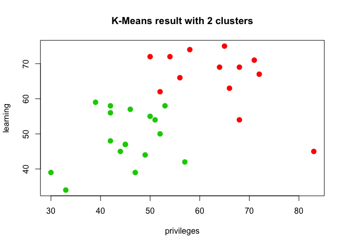
As mentioned before, one of the key decisions to be made when performing K-Means clustering is to decide on the numbers of clusters to use. In practice, there is no easy answer and it’s important to try different ways and numbers of clusters to decide which options is the most useful, applicable or interpretable solution. In the plot above, we randomly chose the number of clusters to be 2 for illustration purposes only. However, one solution often used to identifiy the optimal number of clusters is called the Elbow method and it involves observing a set of possible numbers of clusters relative to how they minimise the within-cluster sum of squares. In other words, the Elbow method examines the within-cluster dissimilarity as a function of the number of clusters. Below is a visual representation of the method:
# Check for the optimal number of clusters given the data

mydata <- dat
wss <- (nrow(mydata)-1)*sum(apply(mydata,2,var))
  for (i in 2:15) wss[i] <- sum(kmeans(mydata,
                                       centers=i)$withinss)
plot(1:15, wss, type="b", xlab="Number of Clusters",
     ylab="Within groups sum of squares",
     main="Assessing the Optimal Number of Clusters with the Elbow Method",
     pch=20, cex=2)
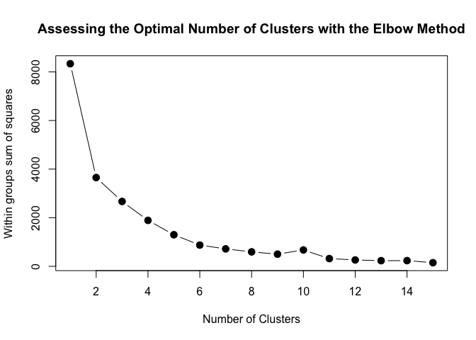
With the Elbow method, the solution criterion value (within groups sum of squares) will tend to decrease substantially with each successive increase in the number of clusters. Simplistically, an optimal number of clusters is identified once a “kink” in the line plot is observed. As you can grasp, identifying the point in which a “kink” exists is not a very objective approach and is very prone to heuristic processes.
But from the example above, we can say that after 6 clusters the observed difference in the within-cluster dissimilarity is not substantial. Consequently, we can say with some reasonable confidence that the optimal number of clusters to be used is 6.
Assuming this assertion is valid, we can go on and apply the identified number of clusters onto the K-Means algorithm and plot the results:
# Perform K-Means with the optimal number of clusters identified from the Elbow method
set.seed(7)
km2 = kmeans(dat, 6, nstart=100)

# Examine the result of the clustering algorithm
km2
## K-means clustering with 6 clusters of sizes 4, 2, 8, 6, 8, 2
##
## Cluster means:
##   privileges learning
## 1   54.50000   71.000
## 2   75.50000   49.500
## 3   47.62500   45.250
## 4   67.66667   69.000
## 5   46.87500   57.375
## 6   31.50000   36.500
##
## Clustering vector:
##  [1] 6 5 4 3 1 3 5 5 4 3 5 3 3 2 1 1 4 4 5 2 6 5 3 5 3 4 1 3 4 5
##
## Within cluster sum of squares by cluster:
## [1]  71.0000 153.0000 255.3750 133.3333 244.7500  17.0000
##  (between_SS / total_SS =  89.5 %)
##
## Available components:
##
## [1] "cluster"      "centers"      "totss"        "withinss"
## [5] "tot.withinss" "betweenss"    "size"         "iter"
## [9] "ifault"
# Plot results
plot(dat, col =(km2$cluster +1) ,
     main="K-Means result with 6 clusters", pch=20, cex=2)
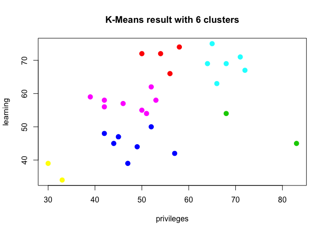
From the results above we can see that there is a relatively well defined set of groups of departments that are relatively distinct when it comes to answering favourably around Privileges and Learning in the survey. It is only natural to think the next steps from this sort of output. One could start to devise strategies to understand why certain departments rate these two different measures the way they do and what to do about it. But we will leave this to another exercise.
In this example we looked at the concept of K-Means clustering and showed a very brief example of its application highlighting the results and the potential concerns that arise from such approaches.