Introduction to Principal Component Analysis (PCA) in Unsupervised Learning Settings
Principal Component Analysis (PCA) is a popular method used in statistical learning approaches.
83 mins reading time
Principal Component Analysis (PCA) is a popular method used in statistical learning approaches. PCA can be used to achieve dimensionality reduction in regression settings allowing us to explain a high-dimensional dataset with a smaller number of representative variables which, in combination, describe most of the variability found in the original high-dimensional data.
PCA can also be used in unsupervised learning problems to discover, visualise an explore patterns in high-dimensional datasets when there is not specific response variable. Additionally, PCA can aid in clustering exercises and segmentation models.
In this article, we’re going to look at PCA as a tool for unsupervised learning, data exploration and visualisation (remembering that visualisation is a key step in the exploratory data analysis process).
In high-dimensional datasets, the ability to visualise patterns among all variables is challenging. One way we can achieve this is by generating two-dimensional scatterplots containing all data points on two of all possible features. However, this technique does not help much when the number of features / variables is large. Consider, for example, the Motor Trend Car Road Test dataset from the 1974 Motor Trend US magazine (this dataset can be found in the library(datasets) package):
# Load necessary libraries
library(datasets)
library(ggplot2)
library(FactoMineR)
library(scales)
library(rgl)
library(knitr)
library(scatterplot3d)

# only display the top 5 records of the mtcars dataset
dta = mtcars
head(dta)
##                    mpg cyl disp  hp drat    wt  qsec vs am gear carb
## Mazda RX4         21.0   6  160 110 3.90 2.620 16.46  0  1    4    4
## Mazda RX4 Wag     21.0   6  160 110 3.90 2.875 17.02  0  1    4    4
## Datsun 710        22.8   4  108  93 3.85 2.320 18.61  1  1    4    1
## Hornet 4 Drive    21.4   6  258 110 3.08 3.215 19.44  1  0    3    1
## Hornet Sportabout 18.7   8  360 175 3.15 3.440 17.02  0  0    3    2
## Valiant           18.1   6  225 105 2.76 3.460 20.22  1  0    3    1
Note that this specific dataset example is only illustrative and is not really a highly-dimensional dataset (cases when the number of features is larger than the number of data points) but it’s an easier example to assimilate the concept.
The mtcars dataset contains 32 observations each representing a specific car model and 11 variables each with a different measure derived from the road test or from the properties of the car.
Even in this basic example, visualising patterns among all variables in the data by running pairwise scatterplots is a challenging endeavour:
# Plot dataset
plot(dta, main="Pairwise Scatterplot of all variables in the mtcars dataset",
     col="blue", cex=0.3, pch=16)
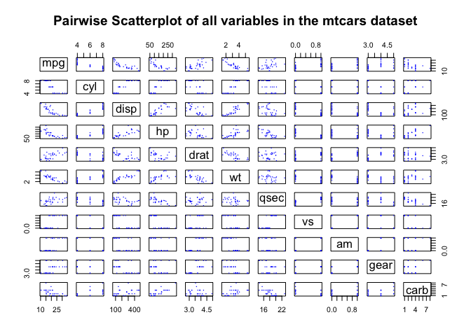
By trying to visualise our dataset of cars (with 11 variables) through the pairwise scatterplot method, we end up having to look through more than 50 individual scatterplots! Now imagine having a dataset with a very large number of variables (hundreds) and trying to visualise and make sense of all of this!
That’s where PCA comes in quite handy.
PCA is a method that allows you to find low-dimensional representations of your data that can explain most of the variation and captures as much information about the dataset as possible. These low-dimensional representations are, essentially, called Principal Components and end up, simplistically speaking, taking the form of new variables. PCA can also be interpreted as low-dimensional linear surfaces that are as closest as possible to each individual observation in a dataset.
PCA computes the first principal component of a set of features / variables by a normalized (centered to mean zero) linear combination of the features that have the largest variance, which after a few mathematical computations, arrives on scores (Z1) for the first principal component. The second principal component (Z2), again, is the linear combination of all features / variables across all data points that have a maximum variance but that are not related with Z1. By making the second principal component uncorrelated to Z1, we are forcing it to be orthogonal (or perpendicular to the direction in which Z1 is projected). The idea here being that if we were to project the PCAs onto a two-dimensional plane, the second PCA would be perpendicular to the first PCA (hence, capturing the variance across both dimensions). Obviously, in a dataset with more than two variables, we can find multiple principal components.
Let’s get back to our example dataset of cars:
# Look at the differences in the mean for each variable
summary(dta)
##       mpg             cyl             disp             hp
##  Min.   :10.40   Min.   :4.000   Min.   : 71.1   Min.   : 52.0
##  1st Qu.:15.43   1st Qu.:4.000   1st Qu.:120.8   1st Qu.: 96.5
##  Median :19.20   Median :6.000   Median :196.3   Median :123.0
##  Mean   :20.09   Mean   :6.188   Mean   :230.7   Mean   :146.7
##  3rd Qu.:22.80   3rd Qu.:8.000   3rd Qu.:326.0   3rd Qu.:180.0
##  Max.   :33.90   Max.   :8.000   Max.   :472.0   Max.   :335.0
##       drat             wt             qsec             vs
##  Min.   :2.760   Min.   :1.513   Min.   :14.50   Min.   :0.0000
##  1st Qu.:3.080   1st Qu.:2.581   1st Qu.:16.89   1st Qu.:0.0000
##  Median :3.695   Median :3.325   Median :17.71   Median :0.0000
##  Mean   :3.597   Mean   :3.217   Mean   :17.85   Mean   :0.4375
##  3rd Qu.:3.920   3rd Qu.:3.610   3rd Qu.:18.90   3rd Qu.:1.0000
##  Max.   :4.930   Max.   :5.424   Max.   :22.90   Max.   :1.0000
##        am              gear            carb
##  Min.   :0.0000   Min.   :3.000   Min.   :1.000
##  1st Qu.:0.0000   1st Qu.:3.000   1st Qu.:2.000
##  Median :0.0000   Median :4.000   Median :2.000
##  Mean   :0.4062   Mean   :3.688   Mean   :2.812
##  3rd Qu.:1.0000   3rd Qu.:4.000   3rd Qu.:4.000
##  Max.   :1.0000   Max.   :5.000   Max.   :8.000
Remember that one of the criteria for one to use PCA is to center variables to have mean zero. This is so Principal Components are not affected by the differences in scales found across all different variables in the data. For example, note how the mean for disp (displacement in cubic inches) is very different from the mean of say carb (number of carburettors) for example. If we do not scale our variables, the Principal Components in this case would be significantly influenced by the disp variable.
Let’s run a Principal Component Analysis on the cars dataset:
# Run Principal Component on the data
PC_res = PCA(dta, scale.unit=TRUE, ncp = dim(dta)[2], graph=FALSE)
summary(PC_res)
##
## Call:
## PCA(X = dta, scale.unit = TRUE, ncp = dim(dta)[2], graph = FALSE)
##
##
## Eigenvalues
##                        Dim.1   Dim.2   Dim.3   Dim.4   Dim.5   Dim.6
## Variance               6.608   2.650   0.627   0.270   0.223   0.212
## % of var.             60.076  24.095   5.702   2.451   2.031   1.924
## Cumulative % of var.  60.076  84.172  89.873  92.324  94.356  96.279
##                        Dim.7   Dim.8   Dim.9  Dim.10  Dim.11
## Variance               0.135   0.123   0.077   0.052   0.022
## % of var.              1.230   1.117   0.700   0.473   0.200
## Cumulative % of var.  97.509  98.626  99.327  99.800 100.000
##
## Individuals (the 10 first)
##                       Dist    Dim.1    ctr   cos2    Dim.2    ctr   cos2
## Mazda RX4         |  2.234 | -0.657  0.204  0.087 |  1.735  3.551  0.604 |
## Mazda RX4 Wag     |  2.081 | -0.629  0.187  0.091 |  1.550  2.833  0.555 |
## Datsun 710        |  2.987 | -2.779  3.653  0.866 | -0.146  0.025  0.002 |
## Hornet 4 Drive    |  2.521 | -0.312  0.046  0.015 | -2.363  6.584  0.879 |
## Hornet Sportabout |  2.456 |  1.974  1.844  0.646 | -0.754  0.671  0.094 |
## Valiant           |  3.014 | -0.056  0.001  0.000 | -2.786  9.151  0.855 |
## Duster 360        |  3.187 |  3.003  4.264  0.888 |  0.335  0.132  0.011 |
## Merc 240D         |  2.841 | -2.055  1.998  0.523 | -1.465  2.531  0.266 |
## Merc 230          |  3.733 | -2.287  2.474  0.375 | -1.984  4.639  0.282 |
## Merc 280          |  1.907 | -0.526  0.131  0.076 | -0.162  0.031  0.007 |
##                    Dim.3    ctr   cos2
## Mazda RX4         -0.601  1.801  0.072 |
## Mazda RX4 Wag     -0.382  0.728  0.034 |
## Datsun 710        -0.241  0.290  0.007 |
## Hornet 4 Drive    -0.136  0.092  0.003 |
## Hornet Sportabout -1.134  6.412  0.213 |
## Valiant            0.164  0.134  0.003 |
## Duster 360        -0.363  0.656  0.013 |
## Merc 240D          0.944  4.439  0.110 |
## Merc 230           1.797 16.094  0.232 |
## Merc 280           1.493 11.103  0.613 |
##
## Variables (the 10 first)
##                      Dim.1    ctr   cos2    Dim.2    ctr   cos2    Dim.3
## mpg               | -0.932 13.143  0.869 |  0.026  0.026  0.001 | -0.179
## cyl               |  0.961 13.981  0.924 |  0.071  0.191  0.005 | -0.139
## disp              |  0.946 13.556  0.896 | -0.080  0.243  0.006 | -0.049
## hp                |  0.848 10.894  0.720 |  0.405  6.189  0.164 |  0.111
## drat              | -0.756  8.653  0.572 |  0.447  7.546  0.200 |  0.128
## wt                |  0.890 11.979  0.792 | -0.233  2.046  0.054 |  0.271
## qsec              | -0.515  4.018  0.266 | -0.754 21.472  0.569 |  0.319
## vs                | -0.788  9.395  0.621 | -0.377  5.366  0.142 |  0.340
## am                | -0.604  5.520  0.365 |  0.699 18.440  0.489 | -0.163
## gear              | -0.532  4.281  0.283 |  0.753 21.377  0.567 |  0.229
##                      ctr   cos2
## mpg                5.096  0.032 |
## cyl                3.073  0.019 |
## disp               0.378  0.002 |
## hp                 1.960  0.012 |
## drat               2.598  0.016 |
## wt                11.684  0.073 |
## qsec              16.255  0.102 |
## vs                18.388  0.115 |
## am                 4.234  0.027 |
## gear               8.397  0.053 |
The summary output of PCA shows a bunch of results. It displays all 11 Principal Components created which contain the scores and their associated PVEs.
Notice that the first two Principal Components explain 84.17% of the variance in the data. Let’s plot the results:
# Plot the results of the two first Principal Components
biplot(PC_res$ind$coord, PC_res$var$coord, scale=0, cex=0.7, main="Biplot for the first two Principal Components", xlab = "First Principal Component (explains ~60%)", ylab="Second Principal Component (explains ~24%)")
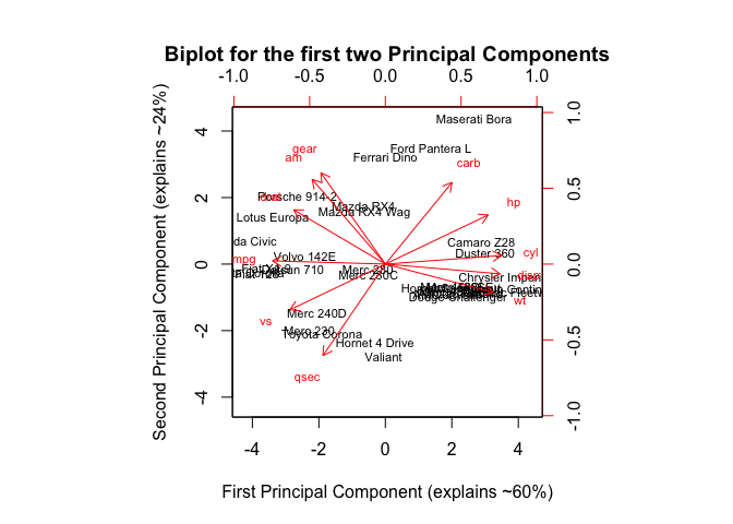
The graph above displays the first two principal components which explain more than 84% of the variance in the cars dataset. The black car names represent the scores for the first two principal components. The red arrows represent the first two principal components loading vectors.
For example, we can see that the first PC (horizontal axis) places more positive weight on variables such as cyl (number of cylinders in a car), disp(displacement in cubic inches of a car) and places negative weights on variables such as mpg (miles per gallon). So we could say that the first PC places cars that are ‘powerful and heavy’ on the right side and places cars that are ‘economical’ and ‘versatile’ on the left side.
The second PC (vertical axis) places positive weight on variables such as gear (number of forward gears a car has) and am (transmission type a=auto and m=manual) and negative weight on variables such as qsec (time in seconds it takes for a car to travel 1/4 mile). So we could argue that the second PC places cars that are ‘manual with lots of gears’ on the top and cars that are ‘more classic-looking and slower’ on the bottom.
Pick the Maseratti Bora which is located on the upper right hand corner of our biplot. According to our interpretation, cars placed on the top and to the left of the graph, should be ‘powerful and heavy’ (right side) and ‘manual with lots of gears’ (top side). As car lovers would know, a Maseratti is a sports car, and it’s a powerful car. Conversely, a Toyota Corona (positioned on the left lower corner of our biplot) is a more versatile and slower car.
We have identified that the first two PC explain more than 84% of the variance in the data.
However, how many Principal Components can be or are created? In general, the number of Principal Components created will be the minimum value found of either (n-1) where n is the number of data points in a dataset or (p) where p is the number of variables in your data. So for example, in our cars dataset, the minimum value between 31 (number of observations - 1) and 11 (number of variables in the cars dataset) is the latter (11). So the expected number of Principal Components will be 11.
# Plot the rotation matrix with the coordinates
PC_res$var$coord
##           Dim.1       Dim.2       Dim.3        Dim.4       Dim.5
## mpg  -0.9319502  0.02625094 -0.17877989 -0.011703525  0.04861531
## cyl   0.9612188  0.07121589 -0.13883907 -0.001345754  0.02764565
## disp  0.9464866 -0.08030095 -0.04869285  0.133237930  0.18624400
## hp    0.8484710  0.40502680  0.11088579 -0.035139337  0.25528375
## drat -0.7561693  0.44720905  0.12765473  0.443850788  0.03655308
## wt    0.8897212 -0.23286996  0.27070586  0.127677743 -0.03546673
## qsec -0.5153093 -0.75438614  0.31929289  0.035347223 -0.07783859
## vs   -0.7879428 -0.37712727  0.33960355 -0.111555360  0.28340603
## am   -0.6039632  0.69910300 -0.16295845 -0.015817187  0.04244016
## gear -0.5319156  0.75271549  0.22949350 -0.137434658  0.02284570
## carb  0.5501711  0.67330434  0.41858505 -0.065832458 -0.17079759
##            Dim.6         Dim.7         Dim.8         Dim.9      Dim.10
## mpg   0.05004636  0.1352413926  0.2643640975  0.0654243559 -0.03177274
## cyl  -0.07753399  0.0210655949  0.0809209881  0.0149987209  0.19307910
## disp  0.15463426  0.0788163447 -0.0004004013  0.0550781718 -0.01126416
## hp   -0.03286009 -0.0005501946  0.0779528673 -0.1598347609 -0.05653171
## drat -0.11246761  0.0077674570 -0.0112861725 -0.0130185049  0.02315201
## wt    0.21387027 -0.0076013843  0.0030050869  0.0997869332 -0.02153254
## qsec  0.15201955  0.0183928603  0.0812768533 -0.1466631306  0.06174396
## vs   -0.08924701 -0.0977488250 -0.0090921558  0.0995327801  0.03627885
## am    0.26257362 -0.2159989575  0.0209456686 -0.0131580558  0.04055512
## gear  0.11203788  0.2225426856 -0.1178452002 -0.0004815997  0.04877625
## carb -0.08441920 -0.0642155284  0.1386968855  0.0473652092 -0.01648332
##            Dim.11
## mpg  -0.018543702
## cyl  -0.020889557
## disp  0.098082614
## hp   -0.038082296
## drat -0.005869197
## wt   -0.084251143
## qsec  0.026927434
## vs    0.001249351
## am    0.004428008
## gear -0.007944389
## carb  0.047451368
Above you can see that there are 11 distinct principal components as expected with their associated score vectors.
Also, from performing PCA, one may wonder how much information is lost by projecting a ‘wide’ dataset onto a few principal components? The answer here is in the Proportion of Variance Explained (PVE) by each Principal Component, which is always a positive quantity that explains the variance of each Principal Component. The PVE is a positive quantity and the cumulative sum of PVEs will be 100%. So, once we plot the Principal Components, it’s always relevant to display the PVE of each Principal Component.
The next natural question is how many Principal Components should one consider? In general, the number of Principal Components in a dataset will be the minimum of either (n-1) where n is the number of data points or (p) where p is the number of variables in your data.
There is one technique to decide on the number of principal components one should use (for explaining most of the variance found in the data) and this is called the scree plot. In essence, a scree plot is a graph that displays the PVE on the vertical axis and the number of principal components found. And the way one chooses the number of principal components is by eyeballing the scree plot and identifying a point at which the proportion of variance explained by each subsequent principal component drops off (similar to the elbow method in K-means when you are trying to find the number of clusters to use).
Let’s plot the PVE explained by each component from our PCA:
# Plot scree plot of the PCs after calculating PVEs
pve = PC_res$eig[1]/sum(PC_res$eig[1])
pc = seq(1,11)
plot_dta = cbind(pc, pve)

ggplot(data=plot_dta, aes(x=pc, y=unlist(pve), group=1)) +
    geom_line(size=1.5) +
    geom_point(size=3, fill="white") +
    xlab("Principal Components") +
    ylab("Proportion of Variance Explained") +
    scale_x_continuous(breaks = c(1:11), minor_breaks = NULL) +
    scale_y_continuous(labels=percent) +
    ggtitle("Scree Plot for Principal Components and Variance")
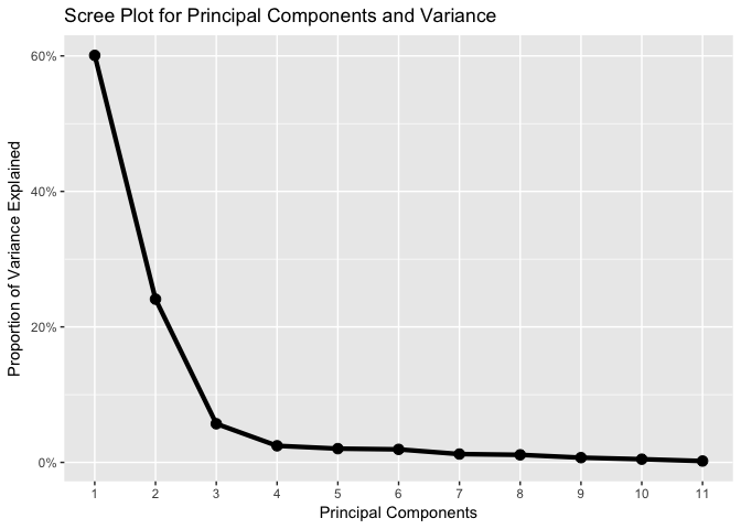
We can see from the scree plot above that the point at which the proportion of variance explained by each subsequent principal component drops off is from the 3rd principal component.
Let’s now plot the first three principal components in an interactive 3D scatterplot (you can click on the graph and drag it around to observe each individual point in different angles. You can also zoom in and out using your mouse scroll wheel):
# Plot 3D PCA after defining the 3 dimensions from PCA

dims = as.data.frame(PC_res$ind$coord)
dims_3 = dims[,c(1:3)]
plot3d(dims_3$Dim.1, dims_3$Dim.3, dims_3$Dim.2, type="s", aspect=FALSE, col="blue", size=1, main="3D plot of the first three Principal Components of the mtcars dataset", sub="Click on and drag it around or zoom in or out to see it in different angles", xlab="First PC (~60%)", ylab="Third PC (~6%)", zlab="Second PC (~24%)")
text3d(dims_3$Dim.1, dims_3$Dim.3, dims_3$Dim.2,row.names(dims_3), cex=0.7, adj=c(1,1))
You must enable Javascript to view this page properly.
Next, we could use the results of the PCA in a supervised learning work (in regression or classification). We could also continue and perform clustering analysis using the results of the PCA to create specific segments of cars that are similar in some ways.
In this article we saw what PCA is in the context of unsupervised statistical learning approaches and how one can perform PCA in a dataset and then briefly interpret its results. As mentioned, PCA can also be used to perform regression models using the principal component scores as features and the use of PCA can lead to a more robust model since most of the important factors in a dataset are concentrated in its first principal components.