Time Series Forecasting in R with Google Analytics Data
Data that are obtained in series of points over an equally spaced period of time are generally referred to as Time series data.
30 mins reading time
Data that are obtained in series of points over an equally spaced period of time are generally referred to as Time series data. Monthly retail sales, daily weather forecast, unemployment figures, consumer sentiment surveys, among many others, are classic examples of time series data. In fact, most variables in nature, science, business and many other applications rely on data that can be measured in a fixed time interval.
One of the key reasons time series data are analysed is to understand the past and predict the future. Scientists can use historical data on climate to predict future climate changes. Marketing managers can look at historical sales of a certain product and predict demand in the future.
In the digital world, a great application of time series data can be on the analysis of visitors to a specific website / blog and predict how many users will that blog or page attract in the future.
In this article, we are going to look at a time series dataset pertaining to users visiting this blog. I’ll set up a connection with Google Analytics API in R and bring daily users from mid-Jan 2017 through to mid-May 2017. We’ll then create a forecast to predict the number of users this blog will likely attract. I’ve randomly picked the date range for illustration purposes only.
The idea here is for us to learn how to query data from Google Analytics into R and how to create a time series forecast.
Let’s start by setting up our working directory and load the necessary libraries:
# set working directory
setwd("/Users/FelipeRego/Documents/blog posts/GATimeSeriesInR")

# load the required packages.
library(RGoogleAnalytics) # Library to connect to Google Analytics.
library(ggplot2) # For some initial plots.
library(forecast) # for the time series prediction.
We should now set up our Google Analytics connection. There is a very well-written guide here that I used which explains how to set up Google Analytics and connect using R so I’ll skip most of the details. In essence, it will show you the package needed and how to perform the necessary query in R to pull data from Google Analytics.
But before that, I had to authorise the RGoogleAnalytics package to fetch data from my user’s Google Analytics Account using OAuth2.0. For details, see Auth topic in the package manual here.
With that sorted, I created a file with my token and client ID details and saved in the directory so I could load it here without displaying my credentials to the public:
# Load the token object
load("GATimeSeriesInR_oauth_token")
With the connection via OAuth sorted, I was able to start querying daily time series data from my blog’s users from the Google Analytics API. Below is the initial query that sets the parameters I wanted. In this example, I’m simply pulling users of my blog by day from mid-Jan 2017 to mid-May 2017.
More details can be found of the Google Analytics Developers pages on how to structure different queries to suit other needs here.
# Create a list of the parameters to be used in the Google Analytics query
list_param = Init(start.date = "2017-01-16",
             end.date = "2017-05-14",
             dimensions = "ga:date",
             metrics = "ga:users",
             sort = "ga:date",
             max.results = 10000,
             table.id = "ga:99395442"
             )
Once the list of parameters of my query are set, I can then start querying the Google Analytics API using the QueryBuilder and the GetReportData functions:
# store the results of the Google Analytics query
res = QueryBuilder(list_param)

# get the data from Google Analytics passing query results and oauth
df = GetReportData(res, oauth_token, split_daywise = T)
## Access Token successfully updated
## [ Run 0 of 118 ] Getting data for 2017-01-16
## [ Run 1 of 118 ] Getting data for 2017-01-17
## [ Run 2 of 118 ] Getting data for 2017-01-18
## [ Run 3 of 118 ] Getting data for 2017-01-19
## [ Run 4 of 118 ] Getting data for 2017-01-20
## [ Run 5 of 118 ] Getting data for 2017-01-21
## [ Run 6 of 118 ] Getting data for 2017-01-22
## [ Run 7 of 118 ] Getting data for 2017-01-23
## [ Run 8 of 118 ] Getting data for 2017-01-24
## [ Run 9 of 118 ] Getting data for 2017-01-25
## [ Run 10 of 118 ] Getting data for 2017-01-26
## [ Run 11 of 118 ] Getting data for 2017-01-27
## [ Run 12 of 118 ] Getting data for 2017-01-28
## [ Run 13 of 118 ] Getting data for 2017-01-29
## [ Run 14 of 118 ] Getting data for 2017-01-30
## [ Run 15 of 118 ] Getting data for 2017-01-31
## [ Run 16 of 118 ] Getting data for 2017-02-01
## [ Run 17 of 118 ] Getting data for 2017-02-02
## [ Run 18 of 118 ] Getting data for 2017-02-03
## [ Run 19 of 118 ] Getting data for 2017-02-04
## [ Run 20 of 118 ] Getting data for 2017-02-05
## [ Run 21 of 118 ] Getting data for 2017-02-06
## [ Run 22 of 118 ] Getting data for 2017-02-07
## [ Run 23 of 118 ] Getting data for 2017-02-08
## [ Run 24 of 118 ] Getting data for 2017-02-09
## [ Run 25 of 118 ] Getting data for 2017-02-10
## [ Run 26 of 118 ] Getting data for 2017-02-11
## [ Run 27 of 118 ] Getting data for 2017-02-12
## [ Run 28 of 118 ] Getting data for 2017-02-13
## [ Run 29 of 118 ] Getting data for 2017-02-14
## [ Run 30 of 118 ] Getting data for 2017-02-15
## [ Run 31 of 118 ] Getting data for 2017-02-16
## [ Run 32 of 118 ] Getting data for 2017-02-17
## [ Run 33 of 118 ] Getting data for 2017-02-18
## [ Run 34 of 118 ] Getting data for 2017-02-19
## [ Run 35 of 118 ] Getting data for 2017-02-20
## [ Run 36 of 118 ] Getting data for 2017-02-21
## [ Run 37 of 118 ] Getting data for 2017-02-22
## [ Run 38 of 118 ] Getting data for 2017-02-23
## [ Run 39 of 118 ] Getting data for 2017-02-24
## [ Run 40 of 118 ] Getting data for 2017-02-25
## [ Run 41 of 118 ] Getting data for 2017-02-26
## [ Run 42 of 118 ] Getting data for 2017-02-27
## [ Run 43 of 118 ] Getting data for 2017-02-28
## [ Run 44 of 118 ] Getting data for 2017-03-01
## [ Run 45 of 118 ] Getting data for 2017-03-02
## [ Run 46 of 118 ] Getting data for 2017-03-03
## [ Run 47 of 118 ] Getting data for 2017-03-04
## [ Run 48 of 118 ] Getting data for 2017-03-05
## [ Run 49 of 118 ] Getting data for 2017-03-06
## [ Run 50 of 118 ] Getting data for 2017-03-07
## [ Run 51 of 118 ] Getting data for 2017-03-08
## [ Run 52 of 118 ] Getting data for 2017-03-09
## [ Run 53 of 118 ] Getting data for 2017-03-10
## [ Run 54 of 118 ] Getting data for 2017-03-11
## [ Run 55 of 118 ] Getting data for 2017-03-12
## [ Run 56 of 118 ] Getting data for 2017-03-13
## [ Run 57 of 118 ] Getting data for 2017-03-14
## [ Run 58 of 118 ] Getting data for 2017-03-15
## [ Run 59 of 118 ] Getting data for 2017-03-16
## [ Run 60 of 118 ] Getting data for 2017-03-17
## [ Run 61 of 118 ] Getting data for 2017-03-18
## [ Run 62 of 118 ] Getting data for 2017-03-19
## [ Run 63 of 118 ] Getting data for 2017-03-20
## [ Run 64 of 118 ] Getting data for 2017-03-21
## [ Run 65 of 118 ] Getting data for 2017-03-22
## [ Run 66 of 118 ] Getting data for 2017-03-23
## [ Run 67 of 118 ] Getting data for 2017-03-24
## [ Run 68 of 118 ] Getting data for 2017-03-25
## [ Run 69 of 118 ] Getting data for 2017-03-26
## [ Run 70 of 118 ] Getting data for 2017-03-27
## [ Run 71 of 118 ] Getting data for 2017-03-28
## [ Run 72 of 118 ] Getting data for 2017-03-29
## [ Run 73 of 118 ] Getting data for 2017-03-30
## [ Run 74 of 118 ] Getting data for 2017-03-31
## [ Run 75 of 118 ] Getting data for 2017-04-01
## [ Run 76 of 118 ] Getting data for 2017-04-02
## [ Run 77 of 118 ] Getting data for 2017-04-03
## [ Run 78 of 118 ] Getting data for 2017-04-04
## [ Run 79 of 118 ] Getting data for 2017-04-05
## [ Run 80 of 118 ] Getting data for 2017-04-06
## [ Run 81 of 118 ] Getting data for 2017-04-07
## [ Run 82 of 118 ] Getting data for 2017-04-08
## [ Run 83 of 118 ] Getting data for 2017-04-09
## [ Run 84 of 118 ] Getting data for 2017-04-10
## [ Run 85 of 118 ] Getting data for 2017-04-11
## [ Run 86 of 118 ] Getting data for 2017-04-12
## [ Run 87 of 118 ] Getting data for 2017-04-13
## [ Run 88 of 118 ] Getting data for 2017-04-14
## [ Run 89 of 118 ] Getting data for 2017-04-15
## [ Run 90 of 118 ] Getting data for 2017-04-16
## [ Run 91 of 118 ] Getting data for 2017-04-17
## [ Run 92 of 118 ] Getting data for 2017-04-18
## [ Run 93 of 118 ] Getting data for 2017-04-19
## [ Run 94 of 118 ] Getting data for 2017-04-20
## [ Run 95 of 118 ] Getting data for 2017-04-21
## [ Run 96 of 118 ] Getting data for 2017-04-22
## [ Run 97 of 118 ] Getting data for 2017-04-23
## [ Run 98 of 118 ] Getting data for 2017-04-24
## [ Run 99 of 118 ] Getting data for 2017-04-25
## [ Run 100 of 118 ] Getting data for 2017-04-26
## [ Run 101 of 118 ] Getting data for 2017-04-27
## [ Run 102 of 118 ] Getting data for 2017-04-28
## [ Run 103 of 118 ] Getting data for 2017-04-29
## [ Run 104 of 118 ] Getting data for 2017-04-30
## [ Run 105 of 118 ] Getting data for 2017-05-01
## [ Run 106 of 118 ] Getting data for 2017-05-02
## [ Run 107 of 118 ] Getting data for 2017-05-03
## [ Run 108 of 118 ] Getting data for 2017-05-04
## [ Run 109 of 118 ] Getting data for 2017-05-05
## [ Run 110 of 118 ] Getting data for 2017-05-06
## [ Run 111 of 118 ] Getting data for 2017-05-07
## [ Run 112 of 118 ] Getting data for 2017-05-08
## [ Run 113 of 118 ] Getting data for 2017-05-09
## [ Run 114 of 118 ] Getting data for 2017-05-10
## [ Run 115 of 118 ] Getting data for 2017-05-11
## [ Run 116 of 118 ] Getting data for 2017-05-12
## [ Run 117 of 118 ] Getting data for 2017-05-13
## [ Run 118 of 118 ] Getting data for 2017-05-14
## The API returned 119 results
# re-orders the results
df = df[order(df$date),]

# inspect the first 30 days of users
head(df,30)
##         date users
## 119 20170116    37
## 118 20170117    66
## 117 20170118    65
## 116 20170119    41
## 115 20170120    72
## 114 20170121    24
## 113 20170122    38
## 112 20170123    68
## 111 20170124    74
## 110 20170125    92
## 109 20170126    95
## 108 20170127    97
## 107 20170128    88
## 106 20170129    59
## 105 20170130    97
## 104 20170131   136
## 103 20170201   192
## 102 20170202   150
## 101 20170203   141
## 100 20170204   109
## 99  20170205    84
## 98  20170206   129
## 97  20170207   181
## 96  20170208   192
## 95  20170209   184
## 94  20170210   158
## 93  20170211   107
## 92  20170212   112
## 91  20170213   152
## 90  20170214   200
As you can see from the 30 records above, the only features or variables used are dates and number of users. It’s a very simple dataset but one that serves well to illustrate the time series forecast example.
The GetReportDate function will set the query in motion. In this example, our time series is 120 days long so the query will take a minute or so to run. For longer, more complex queries, expect longer times and beware of API quotas too! The GetReportDate() function also allows us to pass a split_daywise parameter which paginates the results and break it down on a daily basis.
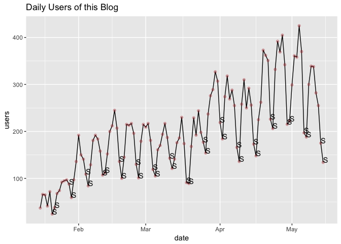
One of the most important steps in time series analysis is to plot your data and inspect it for any patterns and movements in the series. Let’s plot the results our daily users in a time series graph to inspect any trends or seasonality:
# Deal with dates and plot daily users
df$date <- as.Date(df$date, '%Y%m%d')
df$wkd = as.factor(weekdays(df$date))
ggplot( data = df, aes( date, users )) +
  geom_line() +
  ggtitle("Daily Users of this Blog") +
  geom_point(colour = "firebrick", alpha = 0.3) +
  geom_text(aes(label=  ifelse(  substr(wkd,1,1)=="S", substr(wkd,1,1),""  )  ),hjust=0,vjust=0)
# geom_text(data=subset(df, wkd==c("S")), aes(label= ifelse( substr(wkd,1,1) == "S",'' )),hjust=0,vjust=0)
Looking at the plot above with data of daily users of this blog, it seems that users have increased over time. The series starts with less than 100 users and goes up to more than 400 users in one day at a given point. There appears to exist a general upward trend in users. We can also roughly identify peaks and troughs, or ups and downs in the series. This repeating pattern can be linked to seasonal variation. In other words, there appears to exist some level of seasonality in the number of users visiting this blog on a daily basis. We can run a simple box-plot by day of week to try to better visualise this pattern:
# create day of week as factor and plot it
df$wkd = factor(df$wkd, levels = c("Monday", "Tuesday", "Wednesday", "Thursday", "Friday", "Saturday", "Sunday"))
ggplot(df, aes(x=wkd, y=users)) +
  geom_boxplot() +
  geom_jitter(shape=16, position=position_jitter(0.2)) +
  labs(title="User of this blog by Day of Week",x="Day of Week", y = "Users")
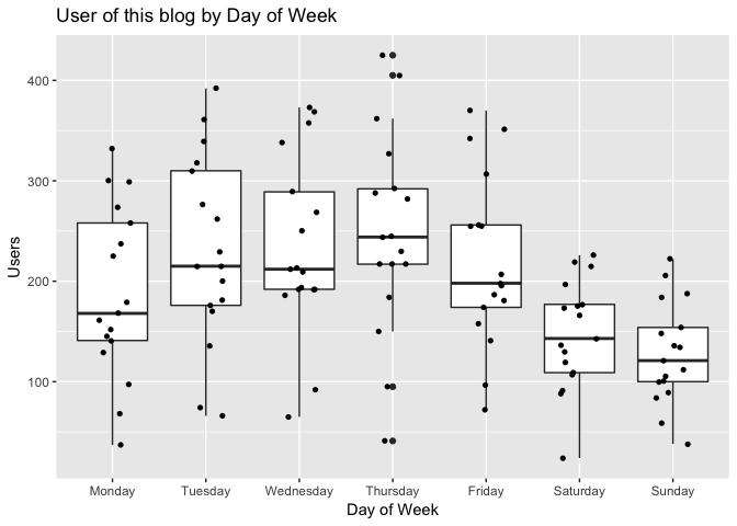
As you can see in the plot above, Tuesdays through to Thursdays are the biggest days in terms of visitors. It attracts a lot of users, with some mid-week days having achieved more than 400 users at some point. In fact, it appears Thursdays contain a large number of outliers compared to other days of the week. Conversely, Saturdays, Sundays and Mondays attract the lowest number of users compared to other days of the week.
So, when we revisit the time series graph above we can now say that the users tend to visit this blog more during the week (peaks on Thursdays) and less during the weekend (troughs on Sunday). This is the seasonal variation we observed earlier.
In time series analysis, we tend to separate (or decompose) the time series data observed into essentially three components: the trend, the seasonal and the irregular.
We do that so we can observe its characteristics and separate the signal from the noise. We decompose time series to identify patterns, make estimates, model the data and improve our ability to understand what is going on and predict future behavior. Decomposing time series allows us to fit a model in the data that best describes its behavior.
The trend component is the long-term direction a time series takes and reflects the underlying level or pattern observed. In our case, the trend is upward which reflects an increasing number of users are visiting the blog.
The seasonal component consists of general effects observed in the data that are consistent in time, magnitude and direction. In our case here, we see frequent positive spikes in users on Wednesdays through to Thursdays for example. Seasonality could be driven by many factors. In retail, seasonality happens in specific dates such as Christmas and Easter. In our blog example, it appears users are visiting more during study / work week and less during the weekend.
The irregular, or also known as the residual, is what remains after we remove both the trend and the seasonal components. It reflects unpredictable movements in the series.
Before we decompose our time series of daily users of this blog, we need to transform our data frame of users we queried directly from Google Analytics into a time series object ts() in R:
# transform data frame into a time series object
df_ts = ts(df$users, frequency = 7)

# decompose time series and plot results
decomp = decompose(df_ts, type = "additive")
print(decomp)
## $x
## Time Series:
## Start = c(1, 1)
## End = c(17, 7)
## Frequency = 7
##   [1]  37  66  65  41  72  24  38  68  74  92  95  97  88  59  97 136 192
##  [18] 150 141 109  84 129 181 192 184 158 107 112 152 200 212 245 207 136
##  [35] 100 145 215 213 217 196 130 101 179 215 209 217 181 119 105 161 170
##  [52] 194 217 187 143 121 141 176 186 230 174  91  89 168 229 192 244 198
##  [69] 177 154 237 276 289 327 307 219 184 274 318 269 288 255 166 136 258
##  [86] 310 250 292 256 173 148 225 262 373 362 351 226 206 332 392 369 405
## [103] 342 215 222 299 361 358 425 370 197 188 300 339 338 282 255 175 134
##
## $seasonal
## Time Series:
## Start = c(1, 1)
## End = c(17, 7)
## Frequency = 7
##   [1]  -7.672869  33.755702  37.032488  48.385429  19.791417 -55.896083
##   [7] -75.396083  -7.672869  33.755702  37.032488  48.385429  19.791417
##  [13] -55.896083 -75.396083  -7.672869  33.755702  37.032488  48.385429
##  [19]  19.791417 -55.896083 -75.396083  -7.672869  33.755702  37.032488
##  [25]  48.385429  19.791417 -55.896083 -75.396083  -7.672869  33.755702
##  [31]  37.032488  48.385429  19.791417 -55.896083 -75.396083  -7.672869
##  [37]  33.755702  37.032488  48.385429  19.791417 -55.896083 -75.396083
##  [43]  -7.672869  33.755702  37.032488  48.385429  19.791417 -55.896083
##  [49] -75.396083  -7.672869  33.755702  37.032488  48.385429  19.791417
##  [55] -55.896083 -75.396083  -7.672869  33.755702  37.032488  48.385429
##  [61]  19.791417 -55.896083 -75.396083  -7.672869  33.755702  37.032488
##  [67]  48.385429  19.791417 -55.896083 -75.396083  -7.672869  33.755702
##  [73]  37.032488  48.385429  19.791417 -55.896083 -75.396083  -7.672869
##  [79]  33.755702  37.032488  48.385429  19.791417 -55.896083 -75.396083
##  [85]  -7.672869  33.755702  37.032488  48.385429  19.791417 -55.896083
##  [91] -75.396083  -7.672869  33.755702  37.032488  48.385429  19.791417
##  [97] -55.896083 -75.396083  -7.672869  33.755702  37.032488  48.385429
## [103]  19.791417 -55.896083 -75.396083  -7.672869  33.755702  37.032488
## [109]  48.385429  19.791417 -55.896083 -75.396083  -7.672869  33.755702
## [115]  37.032488  48.385429  19.791417 -55.896083 -75.396083
##
## $trend
## Time Series:
## Start = c(1, 1)
## End = c(17, 7)
## Frequency = 7
##   [1]        NA        NA        NA  49.00000  53.42857  54.57143  58.42857
##   [8]  66.14286  69.71429  78.85714  81.85714  86.00000  94.85714 109.14286
##  [15] 117.00000 123.28571 126.28571 129.85714 134.42857 140.85714 140.85714
##  [22] 145.71429 148.14286 147.85714 151.85714 155.14286 157.85714 160.71429
##  [29] 169.42857 176.42857 180.57143 178.85714 177.85714 180.00000 180.14286
##  [36] 176.14286 174.57143 173.71429 173.85714 178.71429 178.71429 178.14286
##  [43] 178.14286 176.00000 174.42857 175.00000 172.42857 166.00000 163.85714
##  [50] 163.85714 164.71429 168.14286 170.42857 167.57143 168.42857 167.28571
##  [57] 169.14286 167.28571 159.85714 155.28571 159.14286 166.71429 167.57143
##  [64] 169.57143 173.00000 185.28571 194.57143 204.42857 211.14286 225.00000
##  [71] 236.85714 252.42857 258.42857 262.71429 268.00000 274.00000 271.14286
##  [78] 265.57143 258.14286 250.57143 243.71429 241.42857 240.28571 237.57143
##  [85] 238.14286 238.28571 239.28571 241.00000 236.28571 229.42857 247.00000
##  [92] 257.00000 270.57143 278.14286 286.42857 301.71429 320.28571 319.71429
##  [99] 325.85714 324.57143 323.00000 325.28571 320.57143 316.14286 314.57143
## [106] 317.42857 321.42857 318.85714 314.00000 314.14286 311.00000 308.14286
## [113] 287.71429 271.28571 268.14286 260.42857        NA        NA        NA
##
## $random
## Time Series:
## Start = c(1, 1)
## End = c(17, 7)
## Frequency = 7
##   [1]           NA           NA           NA -56.38542917  -1.21998800
##   [6]  25.32465486  54.96751200   9.53001200 -29.46998800 -23.88963085
##  [11] -35.24257203  -8.79141657  49.03894058  25.25322629 -12.32713085
##  [16] -21.04141657  28.68179772 -28.24257203 -13.21998800  24.03894058
##  [21]  18.53894058  -9.04141657  -0.89855942   7.11036915 -16.24257203
##  [26] -16.93427371   5.03894058  26.68179772  -9.75570228 -10.18427371
##  [31]  -5.60391657  17.75742797   9.35144058  11.89608343  -4.74677371
##  [36] -23.46998800   6.67286915   2.25322629  -5.24257203  -2.50570228
##  [41]   7.18179772  -1.74677371   8.53001200   5.24429772  -2.46105942
##  [46]  -6.38542917 -11.21998800   8.89608343  16.53894058   4.81572629
##  [51] -28.46998800 -11.17534514  -1.81400060  -0.36284514  30.46751200
##  [56]  29.11036915 -20.46998800 -25.04141657 -10.88963085  26.32885654
##  [61]  -4.93427371 -19.81820228  -3.17534514   6.10144058  22.24429772
##  [66] -30.31820228   1.04314226 -26.21998800  21.75322629   4.39608343
##  [71]   7.81572629 -10.18427371  -6.46105942  15.90028511  19.20858343
##  [76]   0.89608343 -11.74677371  16.10144058  26.10144058 -18.60391657
##  [81]  -4.09971489  -6.21998800 -18.38963085 -26.17534514  27.53001200
##  [86]  37.95858343 -26.31820228   2.61457083  -0.07713085  -0.53248800
##  [91] -23.60391657 -24.32713085 -42.32713085  57.82465486  27.18599940
##  [96]  29.49429772 -38.38963085 -38.31820228  13.81572629  33.67286915
## [101]   8.96751200  31.32885654   1.63715486 -45.24677371 -17.17534514
## [106] -10.75570228   5.81572629   2.11036915  62.61457083  36.06572629
## [111] -58.10391657 -44.74677371  19.95858343  33.95858343  32.82465486
## [116] -26.81400060           NA           NA           NA
##
## $figure
## [1]  -7.672869  33.755702  37.032488  48.385429  19.791417 -55.896083
## [7] -75.396083
##
## $type
## [1] "additive"
##
## attr(,"class")
## [1] "decomposed.ts"
plot(decomp)
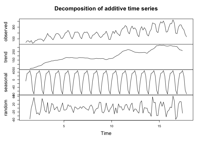
Generally, time series decomposition take the form of either additive or multiplicative. There are also other forms of decomposition, but we’ll not touch on those in this example.
In simplistic terms, additive decompositions are used in time series in which the underlying level of the series fluctuates but the magnitude of the seasonality remains relatively stable. The amplitude of the seasonal and irregular components does not change considerably as the trend level change over time.
On the other hand, multiplicative decompositions are used when the amplitude of the seasonal and irregular increase as the trend increases.
We can observe in the initial time series plot above that the magnitude of the seasonality remains largely stable across the time series which indicates that an additive decomposition would make more sense. In fact, if you inspect our R script above, you can note that we are using an additive decomposition with the decompose() function.
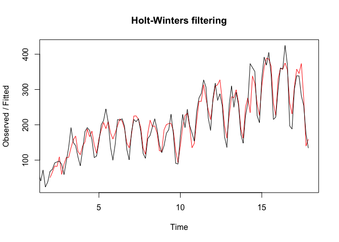
One of our objectives in this exercise is to also try and fit a model that allows us to extrapolate the data and make predictions, forecast of future users of this blog. Obviously, a key assumption in forecasting time series is that the present trend will continue. That is, in the absence of any surprising change or shock, the overall trend should remain similar in the future (at least in the short-term). We’ll also disregard any underlying causes for the patterns observed (i.e. any posts from this blog being featured on a Facebook page which had a lot of visibility and may have driven a lot of users to the blog page, for example).
When we perform forecasting in time series, our intention is to predict some future value given a past history of observations up to a certain point in time. Many considerations need to be taken around the form of exponential smoothing required to fit a time series model. We’ll touch on only one method here for simplicity sake.
So, considering that our time series has seasonality present and uses an additive decomposition, an appropriate smoothing method is the Holt-Winters which uses exponentially weighted moving averages to update estimates.
Let’s fit a predictive model in our time series data:
# apply HoltWinters model in the time series and inspect fit
pred = HoltWinters(df_ts)
print(pred)
## Holt-Winters exponential smoothing with trend and additive seasonal component.
##
## Call:
## HoltWinters(x = df_ts)
##
## Smoothing parameters:
##  alpha: 0.4524278
##  beta : 0.02113644
##  gamma: 0.5593518
##
## Coefficients:
##            [,1]
## a   263.0360074
## b     0.9685586
## s1  -10.4077636
## s2   37.3034145
## s3   34.8402344
## s4   38.7223313
## s5    3.8230454
## s6 -106.7797619
## s7 -122.9210690
As we can see from the model fit above, Holt-Winters’ smoothing is done using three parameters: alpha, beta and gamma. Alpha estimates the trend (or level) component, the beta estimates the slope of the trend component and gamma estimates the seasonal component. These estimates are based on the latest time point in the series and these are the values that will be used for prediction. The values of alpha, beta and gamma range from 0 to 1, where values close to 0 indicates that recent observations have little weight in the estimates.
From the result above, we can see that the smoothing estimate for alpha is 0.4524278, beta is 0.0211364 and gamma is 0.5593518. The value of alpha is around 0.5 which indicates that both short-term, recent observations and historical, more distant observations play a part in the trend estimates of the time series. The value of beta is close to zero which indicates that slope (change in level from one time period to the next) of the trend component remain relatively similar throughout the series. The value of gamma is relatively similar to alpha which indicates that the seasonal estimates are based on both recent and distant observations.
The plot of the model fit (red) and the actual observed values (black) below helps to illustrate the results:
# plot model fit
plot(pred)
We can now extrapolate the model to predict future users of this blog:
# forecast of future users
fcst = forecast.HoltWinters(pred, h=28)
plot.forecast(fcst)
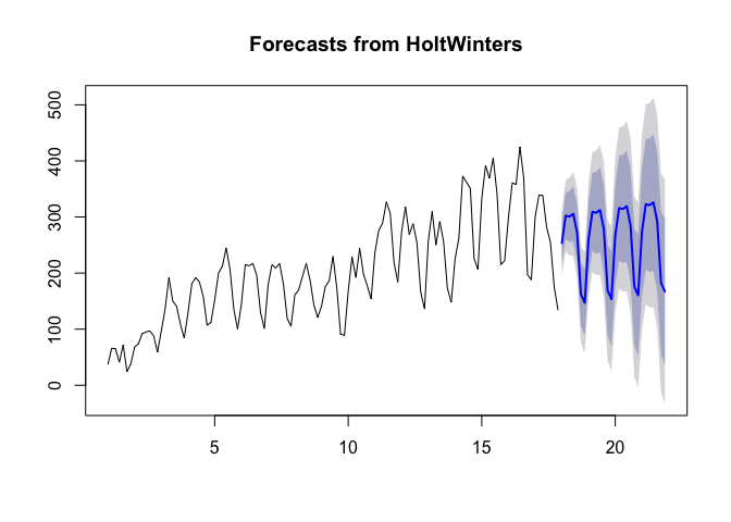
Note from the plot above that the thick, bright blue line represents the forecast of users to this blog over the next month or so. The dark blue shaded area represents the 80% prediction interval and the light blue shaded area represents the 95% prediction interval. As we can see, the model generally illustrates the patterns observed and do a relatively good job in estimating future number of users to this blog.
It’s recommended we check our forecast model accuracy. First let’s look at the Sum of Squared Errors (SSE) which is a measure of how far off our model is from the actual observed data. The squaring is performed to avoid negative values and also to give more weight to larger differences. Values closer to 0 are always better. In our example, we can see that the SSE of our model is 9.8937336\times 10^{4}.
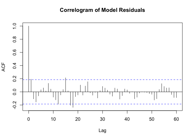
It is also important to check for Autocorrelation. In general, autocorrelation is used to assess whether a correlation exists between the time series and a time lag of that same time series. It’s like taking a copy of that time series multiple times and pasting it every step time ahead and assessing whether a pattern is found. Autocorrelation in the context of time series errors is used to try and find patterns that exist in the residuals. This is what the Correlogram below is trying to do:
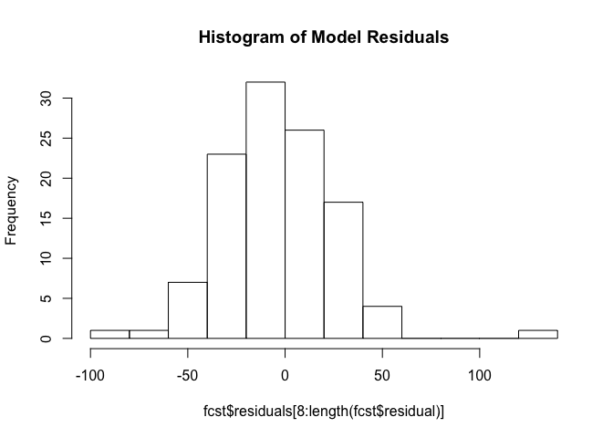
# correlogram and histogram of the model residuals
acf(fcst$residuals[8:length(fcst$residual)], lag=60, main="Correlogram of Model Residuals")
hist(fcst$residuals[8:length(fcst$residual)], breaks=10, main="Histogram of Model Residuals")
Without spending too much time on the Correlogram itself, we can note that while the model works relatively well, it doesn’t do a remarkable job in the early stages of the series as can be seeing in the acf() function autocorrelation results (y axis) at lags 2 and 3.
Additionally, we can see from the histogram of the residuals that the forecast errors are somewhat normally distributed with a presence of some outliers which indicates a relatively good model fit.
Obviously, more tests can and should be performed to test and confirm whether the model is appropriate or can be improved upon, but we’ll leave it at that for now.
In this blog post we briefly described a simplistic approach to bringing Google Analytics data - in this case time series data - into R and created a simple time series forecasting exercise using user of this blog.